Jun 16, 2022

Introduction

I worked on an environment where specific actions are not available at every timestep $t$ when I started deep reinforcement learning.

Let’s illustrate the concept of impossible or unavailable action concretely:

Suppose you want to develop an agent to play Mario Kart. Next, assume that the agent has an empty inventory (no banana 🍌 or anything). The agent can’t execute the action “use the object in the inventory”. Limiting the agent to a meaningful choice of actions will enable it to explore in a smarter way and output a better policy.

Now that you understand the concept of impossible or unavailable action, the natural question is: “How can I manage impossible actions?" 🤔

The first solution I implemented was to assign a negative reward if the agent takes an impossible action. It performed better than not constraining the choice an action, but I was not satisfied with this method as it doesn’t prevent the agent from choosing an impossible action.

Then I decided to use action masking. This method is simple to implement and elegant because it constrains the agent to only take “meaningful” actions.

I have learned that there are many ways to use masks throughout my deep reinforcement learning practice. Masks can be used at any level in the neural network and for different tasks. Unfortunately, few mask implementations for reinforcement learning are available except for this great article by Costa Huang [7].

This blog post’s scope is to explain the concept of masking and illustrate it through figures and code. Indeed, the masks make it possible to model many constraints that we will see as we go along this blog post. Note that the whole process is entirely differentiable. In short, masks are there to simplify your life.

Requirements

A notion of the Markovian decision processes (MDP)
Notions of policy gradient and Q-Learning algorithms
Some knowledge of PyTorch or the basics of numpy
A notion of self-attention. If you want to understand what this concept is, I invite you to read this great article explaining transformers [6]

Action level

Concept:

The primary function of a mask in deep reinforcement learning is to filter out impossible or unavailable actions. For example, in Starcraft II and Dota 2 the total number of actions for each time step is $10^{26}$ and $1,837,080$, respectively. However, each time step's possible action space is a small percentage of the available action space. There are thus two advantages to using masking. The first one is to avoid giving invalid actions to the environment. The second one is that it is a simple method that helps to manage the vast spaces of action by reducing them.

Figure 1 : Visualisation of an action mask at the logit level

Figure 1 illustrates the principle of action masking. The idea behind it is simple, it consists of replacing the logits associated with impossible actions at $-\infty$.

Then, why applying this mask prevents the selection of impossible actions?

Value-based algorithm (Q-Learning) :
In the value-based approach, we select the highest estimated value of the action-value function $Q(s, a)$:
$$ a = \underset{a \in A}{\operatorname{argmax}} Q(s, . ) \text{.} $$
By applying the mask, the Q-values associated with the impossible actions will be equal to $-\infty$, so they will never be the highest value and, therefore, will never be selected.
Policy based algorithm (Policy gradient) :

In the policy-based approach, we sample the action according to the probability distribution at the model’s output: $$ a \sim \pi_{\theta}(. \mid s) \text{.} $$

Therefore, it is necessary to set the probability associated with the impossible action to 0. The logits associated with the impossible action are at$-\infty$ when we apply the mask. We use the softmax function to shift from the logits to the probability domain:

$$ Softmax(\vec{z})_{i} =\frac{e^{z_{i}}}{\sum_{j=1}^{K} e^{z_{j}}} \text { for } i=1, \ldots, K \text { and } \mathbf{z}=\left(z_{1}, \ldots, z_{K}\right) \in \mathbb{R}^{K} \text{.} $$

Considering that we have set the value of logits associated with impossible actions to $-\infty$, the probability of sampling these actions is equal to 0 as $\lim _{x \rightarrow-\infty} e^{x}=0$.

Implementation:

Now let’s practice and implement action masking for a discrete action space and a policy-based algorithm. I used the paper and the action masking code [7] from Costa Huang as a starting point. The idea is simple, we inherit the PyTorch’s Categorical class and add an optional mask argument.

We replace the logits of the impossible action by $-\infty$ when we apply the mask.

However, as we are using float32 we need the minimum value represented in 32 bits. In PyTorch we get it by running torch.finfo(torch.float.dtype).min, which is -3.40e+38.

Finally, for some policy-based approaches such as Proximal Policy Optimization (PPO) [12], it is necessary to compute the probability distribution entropy at the output of the model. In our case, we will compute the entropy of the available actions only.

from typing import Optional

import torch
from torch.distributions.categorical import Categorical
from torch import einsum
from einops import  reduce


class CategoricalMasked(Categorical):
    def __init__(self, logits: torch.Tensor, mask: Optional[torch.Tensor] = None):
        self.mask = mask
        self.batch, self.nb_action = logits.size()
        if mask is None:
            super(CategoricalMasked, self).__init__(logits=logits)
        else:
            self.mask_value = torch.tensor(
                torch.finfo(logits.dtype).min, dtype=logits.dtype
            )
            logits = torch.where(self.mask, logits, self.mask_value)
            super(CategoricalMasked, self).__init__(logits=logits)

    def entropy(self):
        if self.mask is None:
            return super().entropy()
        # Elementwise multiplication
        p_log_p = einsum("ij,ij->ij", self.logits, self.probs)
        # Compute the entropy with possible action only
        p_log_p = torch.where(
            self.mask,
            p_log_p,
            torch.tensor(0, dtype=p_log_p.dtype, device=p_log_p.device),
        )
        return -reduce(p_log_p, "b a -> b", "sum", b=self.batch, a=self.nb_action)

The idea of the following code blocks is to show you how to use the action mask. First, we create dummy logits and also dummy masks with the same shape.

logits_or_qvalues = torch.randn((2, 3), requires_grad=True) # batch size, nb action
print(logits_or_qvalues) 
# tensor([[-1.8222,  1.0769, -0.6567],
#         [-0.6729,  0.1665, -1.7856]])

mask = torch.zeros((2, 3), dtype=torch.bool) # batch size, nb action
mask[0][2] = True
mask[1][0] = True
mask[1][1] = True
print(mask) # False -> mask action 
# tensor([[False, False,  True],
#         [ True,  True, False]])

Then we compare action head with and without masking.

head = CategoricalMasked(logits=logits_or_qvalues)
print(head.probs) # Impossible action are not masked
# tensor([[0.0447, 0.8119, 0.1434], There remain 3 actions available
#         [0.2745, 0.6353, 0.0902]]) There remain 3 actions available

head_masked = CategoricalMasked(logits=logits_or_qvalues, mask=mask)
print(head_masked.probs) # Impossible action are  masked
# tensor([[0.0000, 0.0000, 1.0000], There remain 1 actions available
#         [0.3017, 0.6983, 0.0000]]) There remain 2 actions available

print(head.entropy())
# tensor([0.5867, 0.8601])

print(head_masked.entropy())
# tensor([-0.0000, 0.6123])

We can observe that when we apply the mask, the probabilities associated with impossible actions are equal to $0$. Therefore, our agent will never select impossible actions.

Finally, when we don’t include the impossible actions in the entropy computation, we have consistent values. This corrected entropy computation enable an agent to maximize his exploration only on valid actions.

Such a cool trick!

Feature level

In the paper Hide and seek [8], Open AI introduced masking at the feature extraction level. Each object in the scene is embedded and passed into a masked attention block. Similar to the one proposed in the paper, “Attention is all you need” [5] except that the attention is not computed over time but between the scene’s objects. An object will be masked during the attention computation if it is not in the agent’s field of view.

If this is still unclear to you, don’t worry, we will explain it step by step using figure and code.

Example:

Let’s suppose a grid world where the agent is a panda 🐼. His objective is to eat the watermelon 🍉 and avoid the dragon 🐉 as well as the scorpion 🦂.

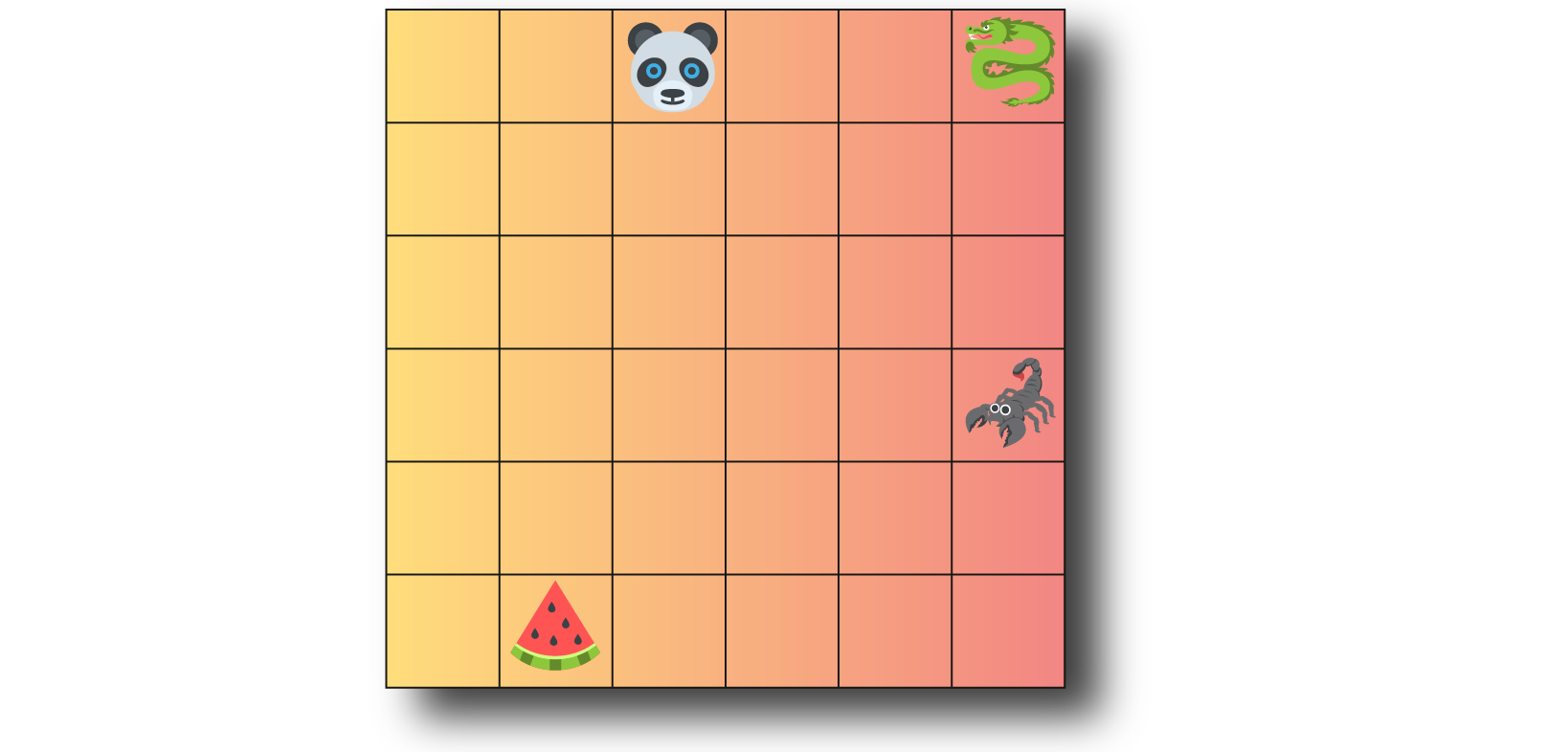
Figure 2 : Grid world with 4 objects: panda 🐼, watermelon 🍉, scorpion 🦂 and dragon 🐉

Each object is represented by a vector of dimension 3. The first component of the vector corresponds to its position on the x-axis in the grid. The second corresponds to its position on the y-axis in the grid. Finally, the vector’s last element corresponds to the type of the object (0: panda 🐼, 1: watermelon 🍉, 2: scorpion 🦂, 3: dragon 🐉).

We can represent this observation as a set as follows: $$ s_{t} = \{ \begin{pmatrix} 3 & 0 & 0 \end{pmatrix} , \begin{pmatrix} 2 & 6 & 1 \end{pmatrix}, \begin{pmatrix} 6 & 4 & 2 \end{pmatrix}, \begin{pmatrix} 6 & 0 & 3 \end{pmatrix} \} $$

Let’s take the panda’s point of view, for this observation he has in his field of view all the elements of the scene. Therefore we can compute the attention score two by two between all the objects in the scene (Illustrated in figure 3).

Figure 3 : Self-attention computation graph when the panda 🐼 sees all other objects

Here, we will implement a tensor representing the observation we have presented above.

Note: Whatever the order of the objects, the self-attention operation is invariant to permutation.

# Observation
# Element set => Panda, Watermelon, Scorpion, Dragon

observation = torch.tensor([[[3, 0, 0], [2, 6, 1], [6, 4, 2], [6, 0, 3]]])
print(observation.size())
# torch.Size([1, 4, 3])  batch size, nb elem set, nb feature

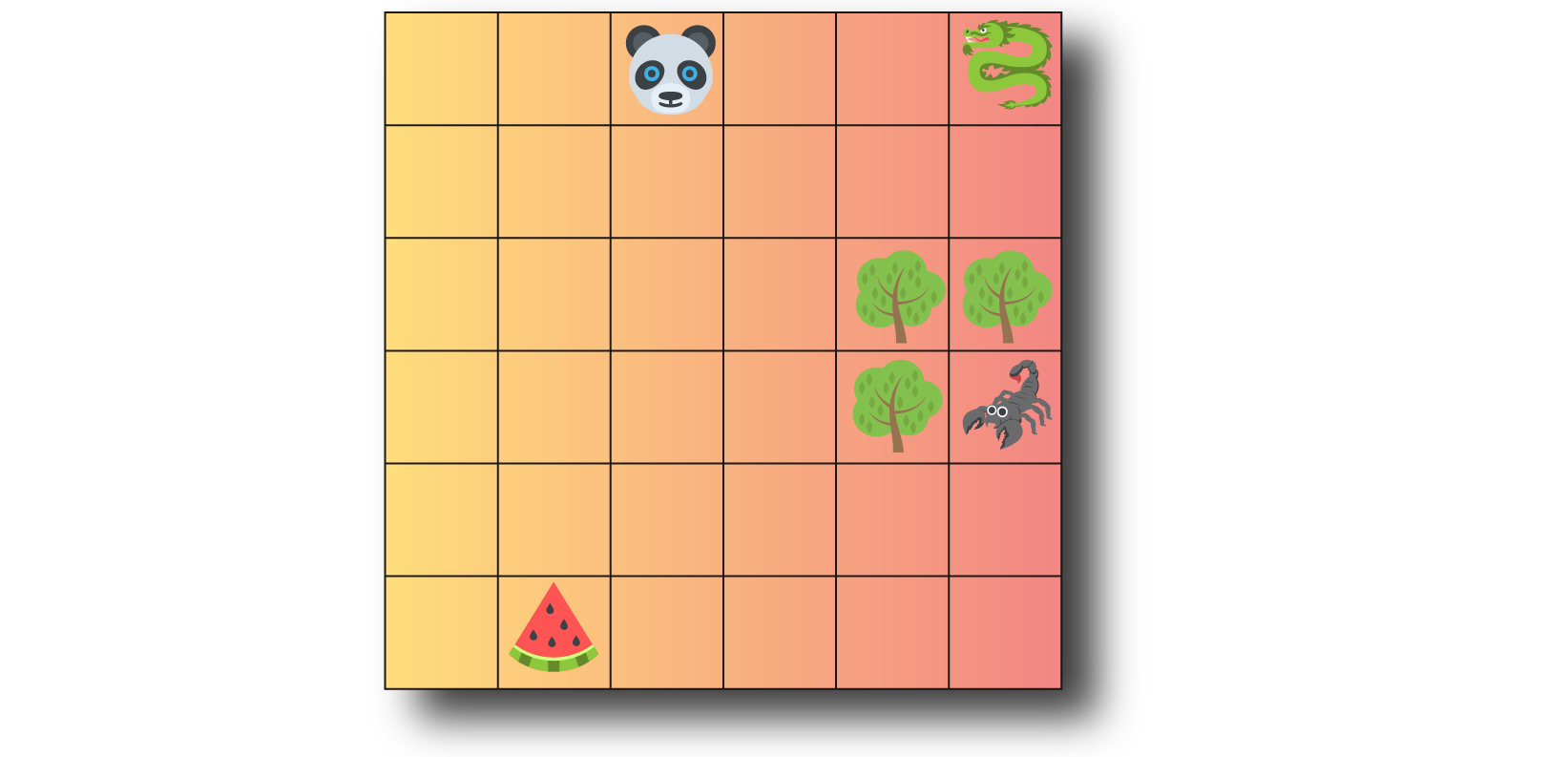
Figure 4 : Grid world with 4 objects: a panda, a watermelon, a scorpion, a dragon and three trees that hide the scorpion

The scene in figure 4 is similar to figure 2; however, 3 trees obstruct the panda’s vision, and he cannot see the scorpion now. In this configuration, attention is calculated as follows: the panda 🐼, watermelon 🍉, and dragon 🐉 compute the attention score between themselves but not with the scorpion 🦂. On the other hand, the scorpion 🦂 calculates his attention scores with himself and all other objects.

Figure 5 : Self attention computation graph when the panda 🐼 see all objects except the scorpion 🦂

Here, we will implement a tensor representing the mask:

# Mask
mask = torch.ones((1, 4), dtype=torch.bool)
# Scorpion is in third position
mask[0][2] = False
print(mask)
# tensor([[ True,  True, False,  True]]) Panda, Watermelon, Scorpion, Dragon
print(mask.size())
# torch.Size([1, 4]) # batch size, nb elem set

Now that we have our inputs for the multi-head attention layer, it is finally time to dive into the rabbit hole. Self-attention is the pairwise interdependence of all elements composing an input.

It is not the scope of this post to explain what attention is and explain in detail each of these operations. If you want dig more into it , I warmly recommend you to read the excellent article of Lilian Weng [11].

Figure 6 : On the left are the operations composing the self-attention, on the right are the operations composing the multi-headed attention layer.

Mathematically we can translate figure 6 into the following equation:

$$ \text { Attention }(Q, K, V, Mask)=\operatorname{softmax}\left(\frac{Mask(Q K^{T})}{\sqrt{d_{k}}}\right) V $$

$$ \text { MultiHead }(Q, K, V, Mask)= \operatorname{Concat}(\text { head } {1}, \ldots, \text { head }_{h}) W^{O} $$

$$ \text { where head }{i} = \text { Attention }(Q W_{i}^{Q}, K W_{i}^{K}, V W_{i}^{V}, Mask) $$

The attention maps result from this block of operation: $\operatorname{softmax}\left(\frac{\operatorname{Mask}\left(Q K^{T}\right)}{\sqrt{d_{k}}}\right) $.

We are interested in these maps because they will enable us to observe the effects of masking.

The masking concept for self-attention is the same as for action masking in the case of policy-based algorithms (by masking the values to $-\infty$ associated with illegal connections between the normalized scalar product and the softmax).

Implementation:

Below you will find the multi-head attention layer code, which is strongly inspired by the Luci drains GitHub [9].

from typing import Optional, Tuple
import torch
from torch import nn, einsum
import torch.nn.functional as F
from einops import rearrange, reduce


class MultiHeadAttention(nn.Module):

    def __init__(self, dim: int, heads: int = 8, dim_head: int = 64):
        super().__init__()
        inner_dim = dim_head * heads
        self.heads = heads
        self.scale = dim_head ** -0.5  # 1/sqrt(dim)
        self.to_qkv = nn.Linear(
            dim, inner_dim * 3, bias=False
        )  # Wq,Wk,Wv for each vector, thats why *3
        self.to_out = nn.Linear(inner_dim, dim)

    def forward(
        self, x: torch.Tensor, mask: Optional[torch.Tensor] = None
    ) -> Tuple[torch.Tensor, torch.Tensor]:
        h = self.heads

        # gets q = Q = Wq matmul x1, k = Wk mm x2, v = Wv mm x3
        qkv = self.to_qkv(x)

        # split into multi head attentions
        q, k, v = rearrange(qkv, "b n (h qkv d) -> b h n qkv d", h=h, qkv=3).unbind(
            dim=-2
        )

        # Batch matrix multiplication by QK^t and scaling
        dots = einsum("b h i d, b h j d -> b h i j", q, k) * self.scale

        if mask is not None:
            mask_value = torch.finfo(dots.dtype).min
            mask = mask[:, None, :, None] * mask[:, None, None, :]
            dots.masked_fill_(~mask, mask_value)

        # follow the softmax,q,d,v equation in the paper
        # softmax along row axis of the attention card
        attn = dots.softmax(dim=-1)

        # product of v times whatever inside softmax
        out = einsum("b h i j, b h j d -> b h i d", attn, v)

        # concat heads into one matrix
        out = rearrange(out, "b h n d -> b n (h d)")
        return self.to_out(out), attn

One of the really cool things about attention is that you can observe the pairwise interdependence (attention score) between each input set element. We will compare the attention map differences with and without the mask in the next two figures. I invite you to move the mouse over the figures to get more details on each element of these attention maps. The second element returned from our MultiHeadAttention layer corresponds to this attention map.

Now, let’s instantiating our multi-head attention layer, we fixed the dim value at 3 because a vector of dimension 3 describes our set elements. We fix the number of heads to 1 for the example. Finally, the size of the heads is fixed at 8.

module = MultiHeadAttention(dim=3, heads = 1,  dim_head = 8)

In figure 2, the panda 🐼 sees all the other objects; it is unnecessary to have a mask at the attention layer’s input.

# Self attention without mask
output_without_mask, attention_map_without_mask = module(observation)
print(output_without_mask.size())
# torch.Size([1, 4, 3])  batch size, nb elem set, nb feature
print(attention_map_without_mask.size())
# torch.Size([1, 1, 4, 4])  batch size, nb head, nb elem set, nb elem set

If you hover the mouse over all the attention map elements, all of them have an attention value that is positive. This means there are no illegal connections for the output representation computation.

Figure 7 : Attention map without mask

In figure 4 the panda 🐼 sees all the other objects except the scorpion 🦂. We will provide the observation and the mask to exclude the scorpion 🦂 from the attention computation for the panda 🐼, the watermelon 🍉 and the dragon 🐉.

# Self attention with mask
output_with_mask, attention_map_with_mask = module(observation, mask)
print(output_with_mask.size())
# torch.Size([1, 4, 3])  batch size, nb elem set, nb feature
print(attention_map_with_mask.size())
# torch.Size([1, 1, 4, 4])  batch size, nb head, nb elem set, nb elem set

If you hover over the scorpion column (key), you’ll observe that the attention score is null except with itself (figure 5). The mask has removed illegal connections between the panda 🐼, the watermelon 🍉, and the dragon 🐉 toward the scorpion 🦂.

Figure 8 : Attention map with mask

We have seen in the two previous figures (7 & 8) that the attention maps are different. Therefore, the outputs will be different. Let’s make some sanity checks.

# Equality test
torch.eq(output_without_mask, output_with_mask)
# False

torch.eq(attention_map_without_mask, attention_map_with_mask)
# False

In this section, we have seen an exciting use of masks in the feature extraction level. The combination of the masks and the multi-head attention layer enbable to build a representation between different entities of a partially observable scene.

Agent level

Finally, the masks last application that I want to present you is to filter agents in a multi-agent configuration in a grid world. Our method implementation comes from the following paper: “Grid-Wise Control for Multi-Agent Reinforcement Learning in Video Game AI” [4].

The abstract of the paper explains well the method of grid control :

“By viewing the state information as a grid feature map, we employ a convolutional encoder-decoder as the policy network. This architecture naturally promotes agent communication because of the large receptive field provided by the stacked convolutional layers. Moreover, the spatially shared convolutional parameters enable fast parallel exploration that the experiences discovered by one agent can be immediately transferred to others”

Notation : $$ \text { State grid: } s \in \mathbb{R}^{w \times h \times c_{s}} $$ $$ \text { Action map : } a \in \mathbb{R}^{w \times h \times c_{a}} $$ $$ \text{Joint action space : } U=U_{1} \times U_{2} \times \cdots \times U_{n_{t}} \text { where } 1,2, \cdots, n_{t} \text { is the set of agents.} $$ $$ \text{Possible action for agent } i \text{ : } \mathbf{u}_{t}= \bigcup_{i=1}^{n_{t}} u_{t}^{i} \text{ , with } u \in U $$ $$ \text{Stochastic joint policy : } \pi\left(\mathbf{u}_{t} \mid s_{t}\right): S \times U \rightarrow[0,1] $$ $$ \text{Actor-Critic loss function : }\nabla_{\theta} J(\theta)=\mathbb{E}_{s, \mathbf{u}}\left[\nabla_{\theta} \log \pi_{\theta}(\mathbf{u} \mid s) A_{\pi}(s, \mathbf{u})\right] $$

The policy network output is an action map where each coordinate is associated with a probability distribution of actions, regardless of the presence or absence of an agent.

The mask’s role will be to filter the grid to compute the joint entropy and joint log probabilities, taking into account only where the agents are.

Figure 9 : High level view of policy network

Implementation:

The action masking code inspired us to implement the code below. Pytorch’s Categorical takes as input a tensor of two dimensions (batch, number of action). However, our input is four (batch, number of action, height, width), so we will have to reshape it. Also, it is necessary to overload the method log_prob to compute all agents joint log probabilities.

The parent method returns a log probability grid. We set the log probabilities in the cells where there is no more agent at 0. Then we compute the joint log probability using the following log property $\log (\prod_{i=1}^{n_{t}} \pi(u_{t}^{i} \mid s_{t})) = \sum_{i=1}^{n_{t}} \log (\pi(u_{t}^{i} \mid s_{t}))$

Finally, we will average the entropy of each probability distribution of the agents present on the grid for the entropy computation.

Note: We could also implement entropy computation on the agents joint action space to maximize the multi-agent system entropy and not each agent independently.

from typing import Optional

import torch
from torch.distributions.categorical import Categorical


class CategoricalMap(Categorical):
    def __init__(self, logits: torch.Tensor, mask: Optional[torch.Tensor] = None):

        self.batch, _, self.height, self.width = logits.size()  # Tuple[int]
        logits = rearrange(logits, "b a h w -> (b h w) a")

        if mask is not None:
            mask = rearrange(mask, "b  h w -> b (h w)")
            self.mask = mask.to(dtype=torch.float32)
        else:
            self.mask = torch.ones(
                (self.batch, self.height * self.width), dtype=torch.float32
            )

        self.nb_agent = reduce(
            self.mask, "b (h w) -> b", "sum", b=self.batch, h=self.height, w=self.width
        )
        super(CategoricalMap, self).__init__(logits=logits)

    def sample(self) -> torch.Tensor:
        action_grid = super().sample()
        action_grid = rearrange(
            action_grid, "(b h w) -> b h w", b=self.batch, h=self.height, w=self.width
        )
        return action_grid

    def log_prob(self, action: torch.Tensor) -> torch.Tensor:
        action = rearrange(
            action, "b h w -> (b h w)", b=self.batch, h=self.height, w=self.width
        )

        log_prob = super().log_prob(action)
        log_prob = rearrange(
            log_prob, "(b h w) -> b (h w)", b=self.batch, h=self.height, w=self.width
        )
        # Element wise multiplication

        log_prob = einsum("ij,ij->ij", log_prob, self.mask)
        log_prob = reduce(log_prob,  "b (h w) -> b", "sum", b=self.batch, h=self.height, w=self.width
        )
        return log_prob

    def entropy(self) -> torch.Tensor:
        entropy = super().entropy()
        entropy = rearrange(
            entropy, "(b h w) -> b (h w)", b=self.batch, h=self.height, w=self.width
        )
        # Element wise multiplication

        entropy = einsum("ij,ij->ij", entropy, self.mask)

        entropy = reduce(
            entropy, "b (h w) -> b", "sum", b=self.batch, h=self.height, w=self.width
        )

        return entropy / self.nb_agent

Let’s take a simple example, our awersome auto-encoder give us a grid of 2x2 size logits with 3 different actions.

action_grid_map = torch.randn(1,3, 2, 2)
print(action_grid_map)
# tensor([[[[ 1.0608,  0.4416],
#           [ 1.2075,  0.0888]],

#          [[ 0.1279,  0.0160],
#           [-1.0273,  0.5896]],

#          [[-0.0016,  0.6164],
#           [ 0.1350,  0.5542]]]])
print(action_grid_map.size())
# torch.Size([1, 3, 2, 2]) batch, nb action, height, width

However, the agents are in positions (0, 0) and (1, 1), so we need our boring mask.

agent_position = torch.tensor([[[True, False],
                               [False, True]]])

print(agent_position)
# tensor([[[ True, False],
#          [False,  True]]])
print(agent_position.size())
# torch.Size([1, 2, 2]) batch, height, width

Let’s instantiate two CategoricalMap one without (boring) mask and the other with.

mass_action_grid = CategoricalMap(logits=action_grid_map)
mass_action_grid_masked = CategoricalMap(logits=action_grid_map, mask=agent_position)

We sample the actions, as you can see that the mask does not influence this stage.

sampled_grid = mass_action_grid.sample()
print(sampled_grid)
# tensor([[[0, 0],
#          [2, 2]]])

sampled_grid_mask = mass_action_grid_masked.sample()
print(sampled_grid_mask)
# tensor([[[1, 1],
#          [2, 1]]])

Suppose we return the same action map associated log probabilities for the Categoricalmap with or without the mask. In that case, you can see that the result is different because without masking, the log probabilities come from the joint probability of all the elements in the action map.

lp = mass_action_grid.log_prob(sampled_grid)
print(lp)
# tensor([-4.0220]) batch

lp_masked = mass_action_grid_masked.log_prob(sampled_grid)
print(lp_masked)
# tensor([-1.5331]) batch

Finally, in the same way, the entropy is different with or without the mask.

entropy = mass_action_grid.entropy()
print(entropy)
# tensor([0.9776]) batch

masked_entropy = mass_action_grid_masked.entropy()
print(masked_entropy)
# tensor([1.0256]) batch

This section has shown how we can use masks in multi-agent reinforcement learning in a grid world. It is also possible to combine this mask with the action mask to manage impossible actions and have a computation of log-probability and entropy by taking into account only the probability distributions of the agents located in the grid.

Conclusion

This article intends to show you different uses of masks in reinforcement learning. When we face more complex environments than toy environments, masks are among the many methods that makes our lives great again.

We have seen through three examples that we can use masks at several neural network or learning process levels. There are many different ways of using a mask. I would be curious to know if you use different methods that those I have presented.

If you have any questions, please do not hesitate to contact me by email or on Twitter.